An efficient load flow solution for distribution system with addition of distributed generation using improved harmony search algorithms

Abstract

The distribution system analysis is very important to know the system condition at any given point of time. This distribution power flow plays an important role. Many power flow techniques have been proposed in the past for distribution power flow (DPF). The implicit Z-bus Gauss–Seidel (GS) method is good when dispersed generations are modelled as PQ nodes in the distribution system but, when dispersed generations are modelled as PV nodes, it leads to divergence problems. In a Newton-like method, a slight change in the execution of the bus-type switching logic leads to an unlike convergence characteristic. Though backward/forward (BW/FW) method is effective and efficient, it slows down under heavy-load condition. Now, with the addition of distributed generation (wind/solar, etc.) at the distribution level, the classical configuration of the distribution system is also changed. This poses a need for more robust and efficient technique. This paper investigates the application of a new algorithm known as improved harmony search (IHS) for DPF. The IHS can determine multiple power flow solutions which fix the limitations of other methods while determining a solution for the highly stressed condition. The results for a standard test system are taken with IHS, Newton–Raphson (NR) and BW/FW method without and with the impact of the wind energy system, to show the potential of the proposed algorithm.

Introduction

The existence of distributed generations (DGs) deviates the unidirectional nature of power flow, and the distribution system no more remains a passive system. The explosion of DGs at distribution levels carried the concept of the active distribution system (ADS). The interconnection of distributed generation sources into the distribution system provides numerous challenges to distribution load flow in terms of modelling of various power delivery and power conversion components. General power delivery components are symbolized by their impedance or admittance, depending on the requirement of solution technique. Moreover, power conversion components can be modelled as negative PQ load, ideal voltage source, PV node or its Norton/Thevenin equivalents.

The steady-state behaviour is the most fundamental calculation of any system. In power systems, this calculation is the steady-state load flow problem, also known as power flow. Several Newton-like methods are developed to solve the problem in [1, 2]. The first model of a backward/forward method for distribution load flow assumes all nodes as PQ since in the distribution system it is assumed that there is no generating bus. Sweeping need not to be calculated, and inversion of Jacobeans as Newton-like methods, resulting in fast convergence, is developed [3]. Firstly, probabilistic load flow is presented in [4] and further reformed and applied to power system load flow problems.

A modified Newton–Raphson (NR) load flow scheme is proposed by [5], which includes generator reactive power limits automatically. This method has slow convergence characteristic but converges monotonically. A slight change in the execution of the bus-type switching logic leads to an unlike convergence characteristic. The ladder network theory [6] and backward/forward method [7] are mostly adopted for load flow study of distribution system due to their computational efficiency and accuracies. An improved backward/forward method is proposed in [8], where the mismatch of a specified voltage and calculated voltage is tested after each backward sweep. But this method arises some limitation if the substation point (specified voltage node) lies in the middle or in between the network rather than on the one side of the network; then the algorithm becomes complex. Hence, the numbering of the nodes should be sequential. The reconstruction of bus injection to branch current (BIBC) and branch current to bus voltage (BCBV) matrix takes place spontaneously by just changing the two elements of the node-by-node sparse matrix (S), reflecting the change in network configuration. But the whole algorithm is applicable to balanced load and balanced system. Also, the convergence speed of the algorithm slows down with higher R/X ratio which is proposed in [9]. [10] presented the behaviour of the transformer in BW/FW-type load flow. The nodal admittance matrix is calculated by primitive admittance matrix using incidence matrix, but in a certain condition as why-delta, zero sequence component cannot update.

The harmony search (HS) algorithm has benefits like easy to implement and fast convergence but still has a disadvantage of precipitate convergence [11], which has been overcome with the help of improved harmony search (IHS) algorithm [12], solving a complex problem of distribution system reconfiguration using HS algorithm. The results are obtained on standard 33-bus and 119-bus system to validate the proposed algorithm. The results are compared with available standard references and found that the proposed algorithm is performing well. The HS algorithm is applied for the optimal allocation of distributed generator, and the total harmonic distortion (THD) analysis has been done to analyse the power quality. The proposed technique is applied on 12-bus unbalance distribution system and is showing that the placement of DG is fast as compared to other techniques [13].

In [14], a genetic algorithm is proposed to solve the power flow problem. An abnormal solution is obtained, which is not possible with the NR method. A genetic algorithm is proposed for distribution system load flow by [15] and also used for integrated AC/DC system load flow in [16]. A real-coded genetic algorithm for load flow solution is proposed [17]. For the placement of various wind distributed generators, a power system optimization (PSO)-based probabilistic load flow model is proposed in [18]. A probabilistic distribution load flow to study the effect of wind turbine generator connected to a distribution system is proposed in [19]. There are three different classes of wind turbine models considered in the distribution system as shown in Fig. 1.

Fig. 1

Different classes of wind turbine models

In constant power factor wind turbine (WT), by controlling the WT trigger angle, reactive power can be adjusted and reactive power can be calculated by knowing the required power factor. In variable reactive power WT, reactive power can be formulated by known active power. Constant voltage WT is handled by considering the connected node as PV node.

In this paper, a constant power factor model is used for modelling the WT. The purpose of the paper is to show the potential of the new proposed algorithm. However, the algorithm is flexible enough, and any other WT model or distribution component model can be conveniently utilized.

The rest of the paper is organized as follows: “Distribution system modelling” section elaborates a brief modelling of the distribution system. “Wind turbine performance model” section describes the wind turbine model which is further considered as DG. The improved harmony search algorithm for power flow analysis is discussed in “Improved harmony search algorithm” section. The results of analysis without and with wind generation as DG are presented in “Results and discussion” section and the conclusions are given in “Conclusions” section.

Distribution system modelling

Distribution system components mainly include two parts: (1) shunt elements such as spot loads, distributed loads, and capacitor banks and (2) series elements such as transformers and line segments. Figure 2 shows a generalized series element model.

Fig. 2

Generalized series element model

An equivalent representation of three-phase conductor with mutual coupling between ground and phases wires is shown in Fig. 3 [6, 20]. And the line segment equations are given below

$$\left[ {\begin{array}{*{20}c} {V_{a} - V_{a}^{'} } \\ {V_{b} - V_{b}^{'} } \\ {V_{c} - V_{c}^{'} } \\ \end{array} } \right] = \left[ {\begin{array}{*{20}c} {Z_{aa - g}^{'} } & {Z_{ab - g}^{'} } & {Z_{ac - g}^{'} } \\ {Z_{ba - g}^{'} } & {Z_{bb - g}^{'} } & {Z_{bc - g}^{'} } \\ {Z_{ca - g}^{'} } & {Z_{cb - g}^{'} } & {Z_{cc - g}^{'} } \\ \end{array} } \right]\left[ {\begin{array}{*{20}c} {I_{a} } \\ {I_{b} } \\ {I_{c} } \\ \end{array} } \right]$$

(1)

Fig. 3

a Mutual coupling between line sections with the ground wire in impedance form; b Transformed network in impedance form

In the admittance form

$$\left[ {\begin{array}{*{20}c} {I_{a} } \\ {I_{b} } \\ {I_{c} } \\ \end{array} } \right] = \left[ {\begin{array}{*{20}c} {Y_{aa - g} } & {Y_{ab - g} } & {Y_{ac - g} } \\ {Y_{ba - g} } & {Y_{bb - g} } & {Y_{bc - g} } \\ {Y_{ca - g} } & {Y_{cb - g} } & {Y_{cc - g} } \\ \end{array} } \right]\left[ {\begin{array}{*{20}c} {V_{a} - V_{a}^{'} } \\ {V_{b} - V_{b}^{'} } \\ {V_{c} - V_{c}^{'} } \\ \end{array} } \right]$$

(2)

Rearrange (2) and calculate $I_{a,}$$I_{b}$ and $I_{c}$. Same procedure can be applied to node $V_{a}^{'} ,V_{b}^{'}$, $V_{c}^{'}$. This results in equivalent series circuit of the line section as shown in Fig. 4, which also includes the impact of coupling.

Fig. 4

Equivalent admittance network of a series line section

So, the three-phase π-model of a line can be written in the nodal frame as

$$\left[ {\begin{array}{*{20}c} {I_{a} } \\ {I_{b} } \\ {I_{c} } \\ {I_{a}^{'} } \\ {I_{b}^{'} } \\ {I_{c}^{'} } \\ \end{array} } \right] = \left[ {\begin{array}{*{20}c} {Y^{abc} + \frac{1}{2}Y_{\text{sn}} } & { - Y^{abc} } \\ { - Y^{abc} } & {Y^{abc} + \frac{1}{2}Y_{\text{sn}} } \\ \end{array} } \right]\left[ {\begin{array}{*{20}c} {V_{a} } \\ {V_{b} } \\ {V_{c} } \\ {V_{a}^{'} } \\ {V_{b}^{'} } \\ {V_{c}^{'} } \\ \end{array} } \right]$$

(3)

where $Y^{abc} = Z^{ - 1,abc}$. The similarity between single-phase and three-phase admittance matrix is that each element being exchanged by a 3 × 3 matrix.

The current injection method can also represent the line charging (shunt capacitance). The charging currents are

$$\begin{aligned} I_{a} = - \frac{1}{2}\left[ {Y_{ab} + Y_{ac} + Y_{an} } \right]V_{a} + \frac{{Y_{ab} }}{2}V_{a} + \frac{{Y_{ac} }}{2}V_{c} \hfill \\ I_{b} = - \frac{1}{2}\left[ {Y_{ab} + Y_{ac} + Y_{an} } \right]V_{b} + \frac{{Y_{ab} }}{2}V_{a} + \frac{{Y_{bc} }}{2}V_{c} \hfill \\ I_{c} = - \frac{1}{2}\left[ {Y_{ab} + Y_{ac} + Y_{an} } \right]V_{c} + \frac{{Y_{ac} }}{2}V_{a} + \frac{{Y_{bc} }}{2}V_{c} \hfill \\ \end{aligned}$$

(4)

Figure 5 shows the capacitance in a three-phase line and its equivalent in current injection form.

Fig. 5

a Capacitances in a 3-ϕ circuit; b equivalent current injections

Wind turbine performance model

The power output from a wind generator is a function of the speed of the wind. The power output changes with the change in wind speed. To compute the power output given from the wind turbine (WT), it is necessary to know about the wind speed and its profile at that particular location in order to quantitatively determine the value of the profile that can be used in the modelling and simulation. A probability distribution function (PDF) is assumed, mathematically which can be represented by (5) [21].

$$f\left( v \right) = \left( {\frac{{kv^{k - 1} }}{{c^{k} }}} \right)\exp^{{ - \left( {\frac{v}{c}} \right)^{k} }}$$

(5)

where k is the shape parameter, c is the scale parameter and v is the wind speed. The cumulative distribution of Weibull distribution is mathematically represented by (6) [21, 22]

$$F\left( V \right) = 1 - \exp^{{ - \left( {\frac{v}{c}} \right)^{k} }} .$$

(6)

Once the uncertain and variable nature of the wind is determined and modelled as a random variable with the help of the probability functions, the output power of the WT may also be written as a random variable through a conversion from wind speed to output power. Ignoring some nonlinearity, the output power from WT can be determined from given wind speed by (7),

$$\left\{ {\begin{array}{ll} {w = 0 ; } & {{\text{for }}v\left\langle {v_{i} \;{\text{and}}\;v} \right\rangle v_{o} } \\ {w = w_{r } \frac{{\left( {v^{2} - v_{i}^{2} } \right)}}{{\left( {v_{r}^{2} - v_{i}^{2} } \right)}};} & {{\text{for}}\;v_{i} \le v \le v_{r} } \\ {w = w_{r } ;} & {{\text{for}}\;v_{r} \le v \le v_{o} } \\ \end{array} } \right\}$$

(7)

where w =output power from wind turbine (typically in kW or MW); w_r= rated power from WECS; v_i=cut-in wind speed (m/s or miles/h); v_r = rated wind speed (m/s or miles/h); v_o = cut-out wind speed (m/s or miles/h).

Figure 6 shows the wind speed Weibull probability distribution function for k = 2 and different values of c.

Fig. 6

Wind speed Weibull probability distribution function

Improved harmony search algorithm in power flow problem

Power flow problem

The rectangular form of power flow problem can be represented as a set of nonlinear equations given below

$$P_{i} = E_{i} \mathop \sum \limits_{j = 1}^{N} \left( {G_{ij} E_{j} - B_{ij} F_{j} } \right) + F_{i} \mathop \sum \limits_{j = 1}^{N} \left( {G_{ij} F_{j} + B_{ij} E_{j} } \right)$$

(8)

$$Q_{i} = F\mathop \sum \limits_{j = 1}^{N} \left( {G_{ij} E_{j} - B_{ij} F_{j} } \right) - E_{i} \mathop \sum \limits_{j = 1}^{N} \left( {G_{ij} F_{j} + B_{ij} E_{j} } \right); i = 1,2, \ldots N$$

(9)

where $E_{i}$ and $F_{i}$ are the real and imaginary parts of ith node voltage. $G_{ij}$ and $B_{ij}$ are the (i, j)th element of bus admittance matrix and N = total number of buses.

For a PQ node, power mismatch can be given as

$$\Delta P_{i} = P_{{i\left( {\text{spe}} \right)}} - P_{{i\left( {\text{cal}} \right)}}$$

(10)

$$\Delta Q_{i} = Q_{{i\left( {\text{spe}} \right)}} - Q_{{i\left( {\text{cal}} \right)}}$$

(11)

where $P_{{i\left( {\text{spe}} \right)}}$ and $P_{{i\left( {\text{cal}} \right)}}$ are the specified and calculated power at ith node.

For a PV node, active power and voltage mismatch will be

$$\Delta P_{i} = P_{{i\left( {\text{spe}} \right)}} - P_{{i\left( {\text{cal}} \right)}}$$

(12)

$$\Delta V_{i} = V_{{i\left( {\text{spe}} \right)}} - V_{{i\left( {\text{cal}} \right)}}$$

(13)

where $V_{{i\left( {\text{spe}} \right)}}$ is the specified voltage at ith PV node and $V_{{i\left( {\text{cal}} \right)}}$ is the calculated voltage and is given by

$$V_{i} = \sqrt {E_{i}^{2} + F_{i}^{2} } .$$

(14)

The power flow problem can be formulated as a minimization-type optimization problem with an objective function Fit as follows

$${\text{Fit}} = \mathop \sum \limits_{i = 2}^{N} \Delta P_{i}^{2} + \mathop \sum \limits_{i = 2}^{N - M} \Delta Q_{i}^{2} + \mathop \sum \limits_{i = 2}^{M} \Delta V_{i}^{2}$$

(15)

where N is the total number of buses. M is the total number of PV buses, considering first bus (i.e. i = 1) as a slack bus.

It is clear that the optimal value of the objective function will be zero (or on the brink of zero). Under a stress or heavily loaded condition when Fit doesn’t go to zero, the method will try to minimize it as much as possible. The unknown variables are: (1) voltage magnitude ($\left| V \right|$) at all buses except slack bus and voltage PV buses with in specified limits $\left[ {V_{ \hbox{min} } , V_{ \hbox{max} } } \right]$; and (2) voltage angle (δ) at all buses within specified limits $\left[ {\delta_{ \hbox{min} } , \delta_{ \hbox{max} } } \right]$.

Improved harmony search algorithm

In general, optimization techniques use gradient information to find the appropriate direction towards an optimal solution. However, a discrete variable cannot have the derivatives. To overcome this, Geem et al. [23] introduced a new meta-heuristic algorithm named harmony search (HS) that is a phenomenon mimicking conceptualized using the musical process of searching for a perfect state of harmony. This coordination in music is analogous to find the optimal solution to an optimization process. An instrumentalist always aims to produce a bit of music with perfect harmony. On the other hand, an optimal solution to an objective function of the optimization problem must be the best solution obtainable to the problem under the given objectives and limited by constraints. Both processes aim to produce the finest or optimum. The harmony search algorithm is used for network optimization [24]. The harmony search algorithm is used for optimal adjustment of PID controller parameter for an interconnected hydrothermal power system, and it shows that controller based on HS has comparatively less time of performance in comparison with genetic algorithm (GA) based controller [25]. The HS method can be successfully applied to various kinds of problems as structural analysis, mechanical component design, water distribution network, medical imaging, games and many others. But, its application in distribution load flow has not yet been investigated.

The various steps of the improved harmony search algorithm are:

• Step 1: Problem formulation: In order to apply harmony search, an objective function should be formulated as

  $${\text{Minimize}}\;F(x)$$

  (16)
  $${\text{Subjected to}};\;x_{i} \in X_{i} ,\;i = 1,2 \ldots N{\text{ or}}\;x_{i}^{L} \le x_{i} \le x_{i}^{U}$$

  (17)

  where $x_{i}$ is the set of variables. $X_{i} = \left[ {x_{i}^{L} ,x_{i}^{U} } \right]$, $x_{i}^{L}$ and $x_{i}^{U}$ are the lower and upper range of variables. N is the number of variables.

• Step 2: Algorithm parameter setting: Once objective function is ready, the parameters of the algorithm should be set with convinced values as harmony memory size (HMS), harmony memory considering rate (HMCR), pitch adjusting rate (PAR), number of improvisation (NI), and fret width (FW). Random length only for a continuous variable is FW, which is generally called as bandwidth (BW).

  Originally fixed values of PAR and BW were used. This fix value leads to higher number of iteration, resulting in slow convergence of the algorithm. There is a varying value for PAR and BW with iterations [26] as:

  $${\text{PAR}}\left( I \right) = {\text{PAR}}_{ \text{min} } + \frac{{\left( {{\text{PAR}}_{ \text{max} } - {\text{PAR}}_{ \text{min} } } \right)}}{\text{NI}} \times I$$

  (18)
  $${\text{BW}}\left( I \right) = {\text{BW}}_{ \text{max} } \exp \left[ {\ln \left( {\frac{{{\text{BW}}_{ \text{max} } }}{{{\text{BW}}_{ \text{min} } }}} \right)\frac{I}{\text{NI}}} \right]$$

  (19)

  where ${\text{PAR}}_{ \text{min} }$ and ${\text{PAR}}_{ \text{max} }$ are the minimum and maximum pitch adjusting rate. ${\text{BW}}_{ \text{max} }$ and ${\text{BW}}_{ \text{min} }$ are maximum and minimum bandwidth. NI is the number of solution vector generation, and I is the generation number.

  In [27, 28], Panigrahi et al. and Das et al. proposed that BW is the standard deviation of the population in each improvising as:

  $${\text{BW}}\left( I \right) = \sigma \left( {x_{i} } \right) = \sqrt {\text{var} \left( {x_{i} } \right)}$$

  (20)

  This modification of PAR and BW called the improved harmony search. This is utilized in this paper.

• Step 3: Harmony memory initialization: Musician’s harmony memory (HM) is an improvisation of many random harmonies. The minimum number of random harmonies should be HMS

  $${\text{HM}} = \left[ {\begin{array}{*{20}c} {x_{1}^{1} } & {x_{2}^{1} } & \ldots & {x_{N - 1}^{1} } & {x_{n}^{1} } \\ {x_{1}^{2} } & {x_{2}^{2} } & \ldots & {x_{N - 1}^{2} } & {x_{N}^{2} } \\ : & : & \ldots & : & : \\ {x_{1}^{{{\text{HMS}} - 1}} } & {x_{2}^{{{\text{HMS}} - 1}} } & \ldots & {x_{N - 1}^{{{\text{HMS}} - 1}} } & {x_{N}^{{{\text{HMS}} - 1}} } \\ {x_{1}^{\text{HMS}} } & {x_{2}^{\text{HMS}} } & \ldots & {x_{N - 1}^{\text{HMS}} } & {x_{N}^{\text{HMS}} } \\ \end{array} } \right].$$

  (21)

• Step 4: Harmony improvisation: A new harmony is generated based on three basic operations expressed as follows: (1) Random selection: The new harmony is generating by randomly picking any value from the total value range $x_{i}^{L} \le x_{i} \le x_{i}^{U}$ with probability of (1-HMCR).

  (2) Memory consideration: A new harmony $x_{i}^{\text{new}}$ is generated by picking up any random value from ${\text{HM}} = \left\{ {x_{i}^{1} , \ldots ,x_{i}^{\text{HMS}} } \right\}$ with probability of HMCR.

  (3) Pitch adjustment: After picking up the new value $x_{i}^{\text{new}}$, it further updated as by a value ($x_{i}^{\text{new}} \leftarrow x_{i}^{\text{new}} \pm \left\{ {r \times {\text{BW}}} \right\}$) with probability of PAR, where r is a random number between (0, 1).

• Step 5: Update memory: In terms of objective, the new better harmony is replaced by worst harmony in HM.

• Step 6: Termination criteria: Process stops when the maximum number of improvisation reached.

  Figure 7 shows the stepwise flowchart of the improved harmony search algorithm.

  Fig. 7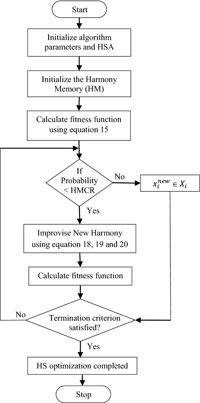

  

  Flowchart of the improved harmony search algorithm

Results and discussion

The studies are performed on a standard 10-bus radial distribution system data [29]. The 10-bus radial distribution system consists of 9 load points. The single-line diagram of 10-bus section of the distribution system with wind generation at bus 10 is shown in Fig. 8.

Fig. 8

Schematic diagram of 10-bus distribution system

Wind power based on wind distribution

The probability of wind speed is calculated as a Weibull curve defined by average wind speed and shape factor k. Generally, k = 2 for inland sites, 3 and 4 for coastal and island sites, respectively [30]. The wind is categorized into “bins” of 1 m/s. The instantaneous wind turbine power for each bin is multiplied by Weibull wind probability giving the net average turbine output power in that bin. The turbine average output power on a continuous 24-h basis is the sum of these powers.

Assuming 11.55 m/s, rated speed of wind turbine and cut-in and cut-out speed is 3 m/s and 20 m/s. The rated power output power of a single turbine is 10 kW, and 75 similar wind turbines are assumed in a farm. Figure 8 shows the wind turbine power (kW) for each bin, Weibull wind probability in percentage and net output power of the turbine. The continuous average power comes 3.07 kW for each wind turbine. So, the total capacity of the wind farm is about 230 kW as shown in Fig. 9.

Fig. 9

Weibull performance calculation of single wind turbine

DLF without wind generation

For the system explained above, the distribution load/power flow studies are conducted by the three methods: (1) NR in rectangular form; (2) BW/FW sweep method [8] and (3) IHS algorithm.

In the study, the slack bus voltage and angle are fixed to 1 per unit and 0°. All buses are considered as PQ bus except one slack bus (bus 1). Table 1 shows the comparative study of voltage (per unit) and angles (°) for base case by all the three methods. The voltage magnitude and angles at various buses remain same with NR and BW/FW. Hence, they are represented by a single column.

Table 1 Voltage magnitude and angles at all buses for the base case

Uniform load increase scenario has been utilized to increase the load as

$$P_{{D {\text{new}}}}^{i} = P_{{D {\text{base}}}}^{i} \left( {1 + \lambda } \right)$$

(22)

$$Q_{{D {\text{new}}}}^{i} = Q_{{D {\text{base}}}}^{i} \left( {1 + \lambda } \right)$$

(23)

where i = 1,2,….n; n = number of load buses. $P_{{D {\text{base}}}}^{i}$ and $Q_{{D {\text{base}}}}^{i}$ are the base case active and reactive power demand at ith bus. λ is the load parameter. The uniform load increase scenario has been utilized for simplicity. However, the user can take any practical load increase scenario.

By gradually increasing the loads, Table 2 shows the voltage (per unit) and angles (°) of 10-bus radial distribution system by all the three methods. Again, voltage and angle remain very nearly same for NR and BW/FW method for loading parameter λ = 0.5. Again increasing the load, the Newton method fails to converge at λ = 1. Table 2 shows the voltage magnitude and angle for λ = 0.5 and 1.

Table 2 Voltage magnitude and angles at all buses for loading parameter 0.5 and 1

Again, increasing the load, both the methods (NR and BW/FW) fail to converge at loading parameter 1.2. Table 3 shows the voltage (per unit) and angles (°) profile with loading factor 1.2 by IHS algorithm.

Table 3 Voltage magnitude and angles at all buses for λ = 1.2

DLF with wind power generation incorporated

By the loss-power sensitive, the appropriate location is found at bus 10. So, a total 230 kW wind generation is considered at bus 10. In this work, wind generation is modelled as negative PQ load. The load/power flow studies are again conducted by the three methods: (1) Newton method (NR) in rectangular form; (2) backward/forward (BW/FW) sweep method; and (3) improved harmony search (IHS) algorithm.

In the study, again the slack bus voltage and the angle are fixed to 1 per unit and 0°. Table 4 shows the comparative study of voltage (per unit) and angles (°) for base case by all the three methods. By gradually increasing the loads, Table 5 shows the voltage magnitude (per unit) and angles (°) for loading parameter, λ = 0.5 and 1.2. The voltage and angle are remained very nearly same for NR and BW/FW method at loading 0.5. At loading 1.2, Newton’s method fails to converge.

Table 4 Voltage magnitude and angles at all buses for the base case

Table 5 Voltage magnitude and angles at all buses for loading parameter 0.5 and 1.2

Again, increasing the load, both the methods (NR and BW/FW) fail to converge at loading parameter 1.5, which has earlier failed at loading 1.2 in “DLF without wind generation” section, it shows the improved load handling capability due to the presence of wind generation. So, due to wind generation, the convergence capability shifts to higher loading side. Table 6 shows the voltage and angle profile with loading parameter 1.5 by IHS algorithm.

Table 6 Voltage magnitude and angles at all buses for λ = 1.5

Conclusions

This work represents the application of improved harmony search algorithm for solving distribution system power flow problem. The algorithm is applied to standard 10-bus distribution system, and the results are compared with conventional NR and BW/FW method. The advantage of the proposed IHS method over conventional methods is its robustness. In many cases, during very heavy loaded condition the NR and BW/FW method fails to provide DLF solution. This method can be used to find the DLF solution in such situations where the NR and BW/FW method fails. The small-scale distributed generation is an attractive architecture for new distribution networks. Hence, in this paper wind generation system is also included in modelling DLF. The model concludes the adequacy analysis of distribution system power flow with significant wind generation. The results for standard 10-bus system demonstrate the potential of the proposed algorithm.

Appendix

A. 1. Wind turbine

B. 1. Harmony search algorithm

Harmony memory size = 55

Harmony memory consideration =  0.98

Pitch adjustment = 0.1 to 0.99

C. 1. 10-Bus radial distribution system

See Table 7.

Table 7 10-bus distribution network system data

References

Baran ME, Wu FF (1989) Optimal sizing of capacitors placed on a radial distribution system. IEEE Trans Power Deliv 4(1):735–743
AlHajri MF, El-Hawary ME (2010) Exploiting the radial distribution structure in developing a fast and flexible radial power flow for unbalanced three-phase networks. IEEE Trans Power Deliv 25(1):378–389
Alinjak T, Pavic I, Trupinic K (2017) Improved three-phase power flow method for calculation of power losses in unbalanced radial distribution network. CIRED Open Access Proc J 2017(1):2361–2365
Huang Y, Xu Q, Yang Y, Jiang X (2018) Numerical method for probabilistic load flow computation with multiple correlated random variables. IET Renew Power Gener 12(11):1295–1303
Sundaresh L, Nagendra Rao PS (2014) A modified Newton–Raphson load flow scheme for directly including generator reactive power limits using complementarity framework. Electr Power Syst Res 109:45–53
Kersting WH (2002) Distribution system modeling and analysis. CRC Press, Boca Raton
Dall’Anese E, Baker K, Summers T (2017) Chance-constrained AC optimal power flow for distribution systems with renewables. IEEE Trans Power Syst 32(5):3427–3438
Chang GW, Chu SY, Wang HL (2007) An improved backward/forward sweep load flow algorithm for radial distribution systems. IEEE Trans Power Syst 22(2):882–884
Abul Wafa AR (2012) A network-topology-based load flow for radial distribution networks with composite and exponential load. Electr Power Syst Res 91:37–43
Kocar I, Lacroix JS (2012) Implementation of a modified augmented nodal analysis based transformer model into the backward forward sweep solver. IEEE Trans Power Syst 27(2):663–670
Sun W, Chang X (2015) An improved harmony search algorithm for power distribution network planning. J Electr Comput Eng 2015:1–6
Srinivasa Rao R, Narasimham SVL, Ramalinga Raju M, Srinivasa Rao A (2011) Optimal network reconfiguration of large-scale distribution system using harmony search algorithm. IEEE Trans Power Syst 26(3):1080–1088
Parizad A, Khazali AH, Kalantar M (2010) Sitting and sizing of distributed generation through Harmony Search Algorithm for improve voltage profile and reeducation of THD and losses, CCECE 2010, Calgary, AB, pp 1–7
Kim H, Samann N, Shin D, Ko B, Jang G, Cha J (2007) A new concept of power flow analysis. J Electr Eng Technol 2(3):312–319
Chakraborty D, Sharma CP, Das B, Abhishek K, Malakar T (2009) Distribution system load flow solution using Genetic Algorithm. In: 2009 international conference on power systems. https://doi.org/10.1109/ICPWS.2009.5442749
Ayan K, Arifoglu U, Kilic U (2011) Integrated AC/DC systems load flow using genetic algorithm. In: 2011 5th international power engineering and optimization conference, pp 404–409. https://doi.org/10.1109/PEOCO.2011.5970380
Kubba H, Mokhlis H (2012) An enhanced RCGA for a rapid and reliable load flow solution of electrical power systems. Int J Electr Power Energy Syst 43(2):304–312
Jain N, Singh SN, Srivastava SC (2014) PSO based placement of multiple wind DGs and capacitors utilizing probabilistic load flow model. Swarm Evol Comput 19:15–24
Ahmed MH, Bhattacharya K, Salama MMA (2013) Probabilistic distribution load flow with different wind turbine models. IEEE Trans Power Syst 28(2):1540–1549
Das JC (2002) Power system analysis: short-circuit load flow and harmonics. Marcel Dekker, Inc., New York
Hetzer J, Yu DC, Bhattarai K (2008) An economic dispatch model incorporating wind power. IEEE Trans Energy Convers 23(2):603–611
Mishra S, Mishra Y, Vignesh S (2011) Security constrained economic dispatch considering wind energy conversion systems. In: 2011 IEEE power and energy society general meeting. https://doi.org/10.1109/PES.2011.6039544
Geem ZW (2009) Music-inspired harmony search algorithm: theory and applications. Springer, Berlin
Ezhilarasi GA, Swarup KS (2012) Network decomposition using Kernighan-Lin strategy aided harmony search algorithm. Swarm Evol Comput 7:1–6
Shivaie M, Kazemi MG, Ameli MT (2015) A modified harmony search algorithm for solving load-frequency control of non-linear interconnected hydrothermal power systems. Sustain Energy Technol Assess 10:53–62
Liu WK, Liu Y, Ye X, He K (2016) Reactive power coordinated optimisation method with renewable distributed generation based on improved harmony search. IET Gener Transm Distrib 10(13):3152–3162
Panigrahi B, Pandi V, Das S, Abraham A (2010) Population variance harmony search algorithm to solve optimal power flow with non-smooth cost function. In: Recent advances in harmony search algorithm 2010, pp 65–75
Das S, Mullick SS, Suganthan PN (2016) Recent advances in differential evolution—an updated survey. Swarm Evol Comput 27:1–30
Baghzouz Y, Ertem S (1990) Shunt capacitor sizing for radial distribution feeders with distorted substation voltages. IEEE Trans Power Deliv 5:650–657
Windcad turbine performance model, USDA IEC 61400-12 Data
Acknowledgements
Not applicable.
Funding
Author information
Authors and Affiliations
Contributions
AT contributed as main author of this work and the efficient techniques to improve the voltage level at distribution by providing the additional distributed generation that has been developed. The work proposed efficient and effective power flow techniques for distribution system. KK supported the main author to identify the problems of for load flow and suggested the work in the direction of additional distributed generation. MAA is the expert in the field of load flow and arranged the research in proper direction with novelty. BK supported in this research work as the content of this work, and also the proofreading of this work as an expert in this field is done. All authors read and approved the final manuscript.
Corresponding author
Ethics declarations
Competing interests
The results in this paper are compared with standard data, and the system performance is enhanced in this research.
Additional information
Publisher's Note
Springer Nature remains neutral with regard to jurisdictional claims in published maps and institutional affiliations.